 Aspecten
 Download (3 GB)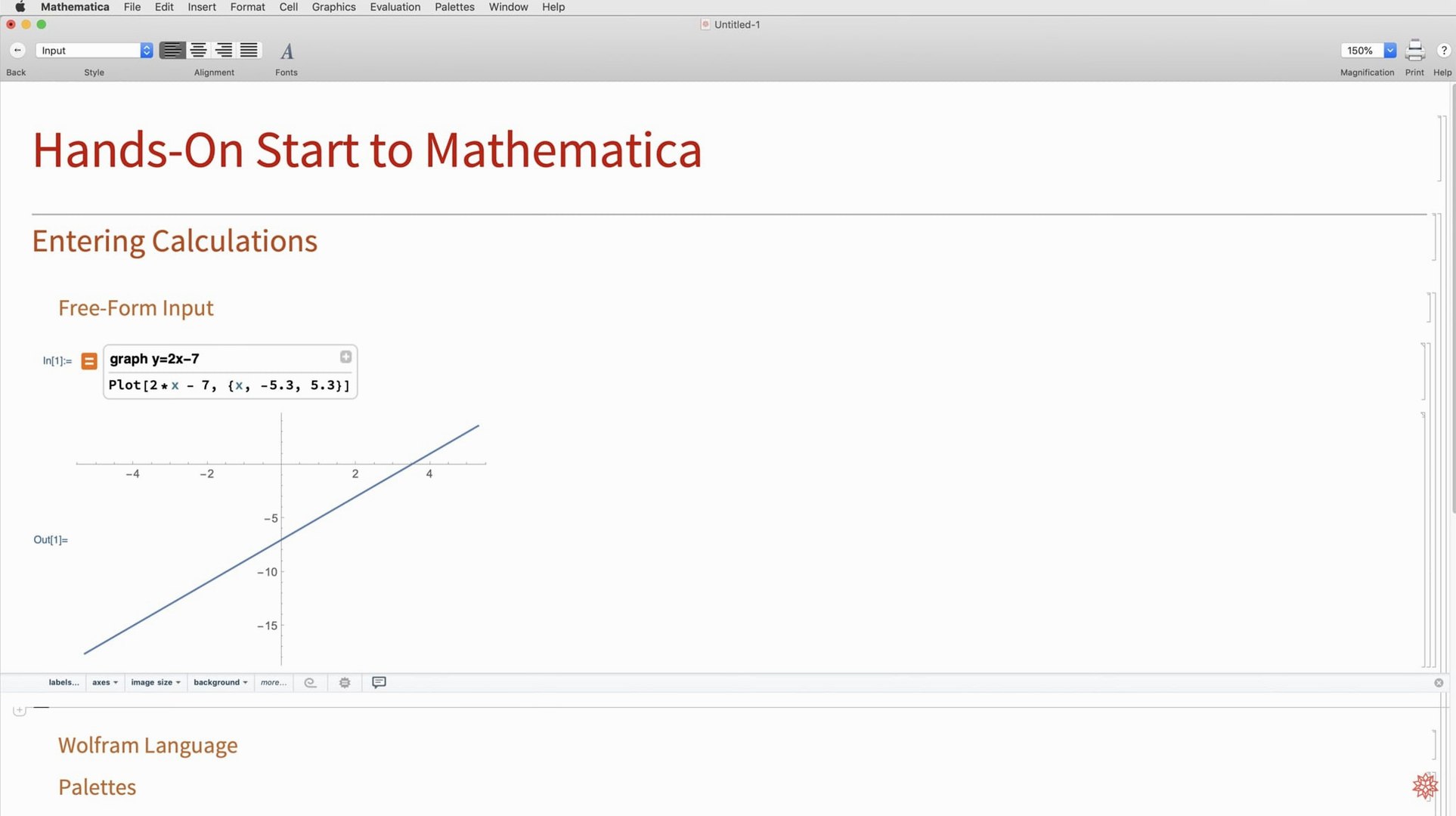
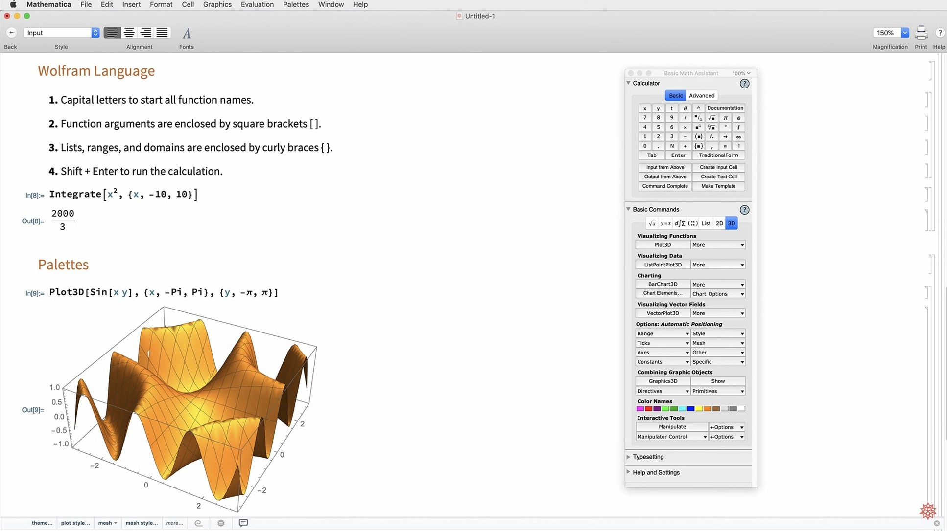
Version 14.3 is the first release built with full dark mode support across notebooks and interface chrome, accompanied by a new set of standard colours tuned for both light and dark environments. The update also brings Hilbert transforms, Lommel functions, and additional matrix decompositions into the symbolic engine.
Symbolic math and thousands of functions without libraries
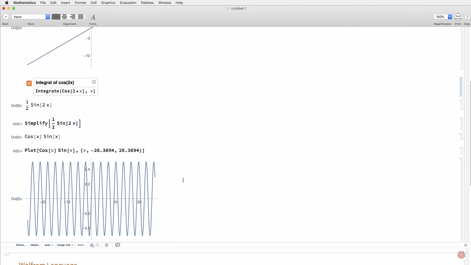
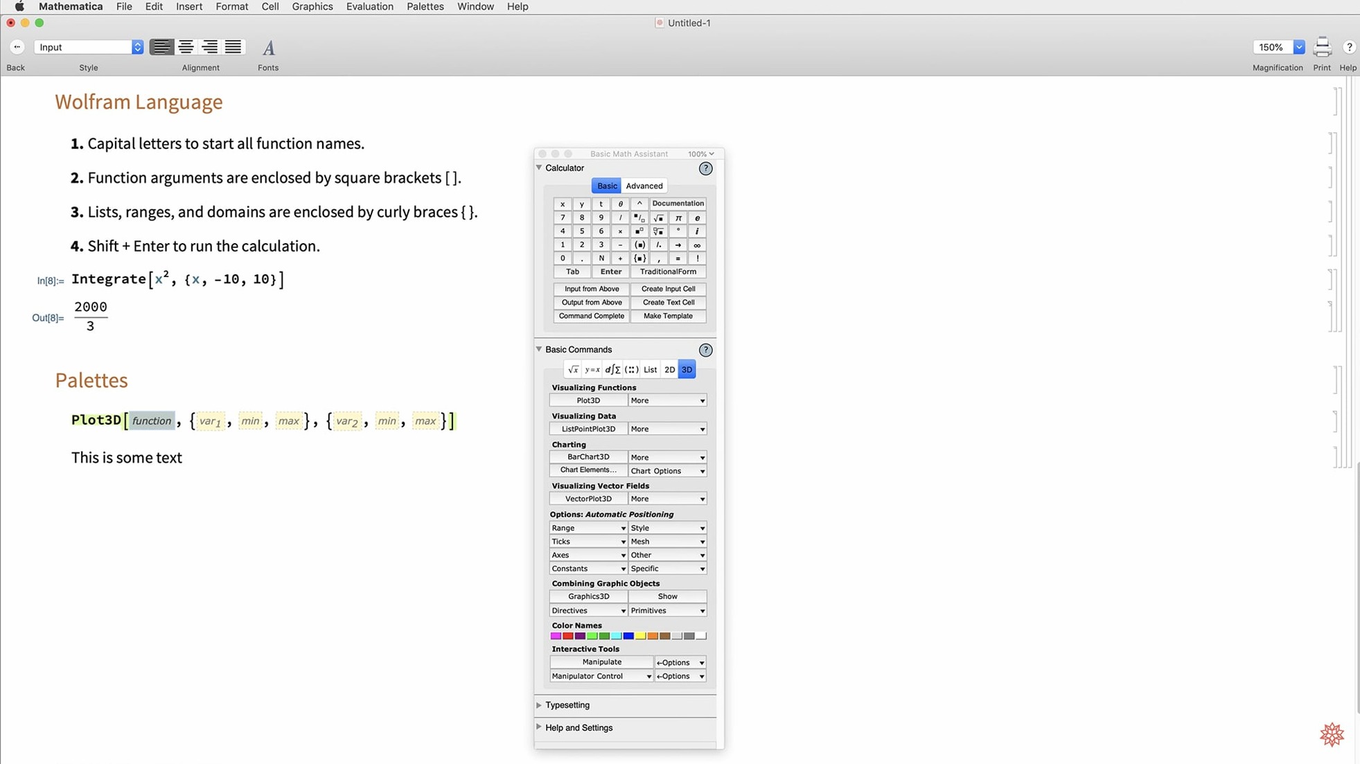
- Symbolic and numerical computation. Mathematica handles equation solving, calculus, linear algebra and probability with exact or arbitrary-precision results. The Wolfram Language gives access to thousands of built-in functions without external libraries.
- Data acquisition and analysis. Tools for importing structured data, cleaning it, applying statistical models, and exporting results sit alongside natural-language input, so you can describe a computation in plain English and get working code back.
- Visualisation. ListFitPlot and updated surface plotting functions join vector-based maps and mesh processing routines in 14.3, making it simpler to produce publication-ready graphics without leaving the notebook.
- Interoperability. Faster Python and R integration, Markdown export, and the new LLMGraph function connect Mathematica sessions to external workflows and language models with less friction.
Deployment and reach
Results can be deployed to multiple local and network formats, from CDF documents to cloud APIs. The 14.3 release also adds geodesic computation, ColumnwiseCombine for data reshaping, and system model validation tools, giving engineers and data scientists a broader set of verified building blocks.
Formatted notebooks that paste math typesetting into Pages and Keynote
Mathematica does not live in a silo. The notebook interface supports copy and paste of formatted text, images, and tables between Mathematica and Pages, Keynote, or Word while preserving mathematical typesetting. Graphics exported as PDF or SVG drop cleanly into vector-editing apps. For developers who prefer writing in a code editor, Wolfram Language scripts with a .wls extension run directly from Terminal, and wolframscript integrates with shell pipelines just as Python or Ruby would.
On macOS, Mathematica respects Dark Mode system-wide, switching notebook chrome and cell styling automatically when the system appearance changes — something 14.3 formalised. It registers itself as a Spotlight-importer, so notebook filenames and text content are searchable without opening the app. You can also use Automator or Shortcuts to launch a Mathematica script that processes a selected file; a common setup is a Finder Quick Action that takes a CSV, runs a ListPlot script, and saves a PNG alongside the original.
Cloud access through a web browser means a notebook started on the desktop continues on an iPad or any machine with a Wolfram Cloud account, with computations running on remote kernels. External data flows in through Import from URLs, REST APIs, or SQL databases, and the new ColumnwiseCombine function in 14.3 helps when you are merging responses from different services into a single rectangular dataset.
Shift-Return evaluates in place, Return starts a new line
One common stumble is treating Mathematica like a calculator with a bigger display. Typing an expression and pressing Return evaluates it and moves to a new line; pressing Shift-Return evaluates the current cell in place. People who miss this distinction end up with notebooks full of unevaluated cells and wonder why nothing ran.
Another is ignoring the difference between immediate assignment = and delayed assignment :=. Writing x = RandomReal[] freezes a single random number into x at assignment time, while x := RandomReal[] gives a fresh value each time x is evaluated. The wrong choice creates bugs that survive for weeks in a notebook before the underlying rule is understood.
Beginners also overuse the natural-language input bar without inspecting the generated code. The Wolfram Language is precise; the natural-language parser is an assistant, not a replacement for learning the syntax. A query like “plot the data in column 2” might produce a ListPlot that runs, but it might also silently drop rows with missing values in a way the user did not intend. Checking the output code line by line is the habit that separates reliable notebooks from fragile ones.
A native ARM build on Apple Silicon and when it can replace Python
Does it run on Apple Silicon Macs? Yes. Version 14.3 includes a native ARM build, and it runs on Intel 64-bit Macs as well. The installer handles the architecture automatically.
Can Mathematica replace my Python or R setup? It can handle many of the same tasks — data wrangling, statistical modelling, machine learning, plotting — but whether it replaces your existing tools depends on your workflow. The 14.3 speed improvements for Python and R integration mean you can call those languages from within a Mathematica session when you need a library that only exists in one ecosystem, without leaving the notebook.
How steep is the learning curve? The basics are shallow: you can plot a function, solve an equation, or import a CSV with a single short expression. The depth comes from the Wolfram Language's functional and pattern-matching features, which take time to internalise. Most people grow into it gradually, starting with numerical work and picking up symbolic and pattern-based programming as their projects demand it.
Does it need a constant internet connection? No. The desktop application runs entirely offline. Cloud features — cloud saving, remote kernels, web deployment — need a connection and a Wolfram Cloud account, but local notebooks and computations work without one.
A workflow: fitting and visualising experimental data
Suppose you have time-series data from a temperature sensor logged as CSV. The file has columns for timestamp, reading, and sensor ID. You want to clean the data, fit a decay model, and produce a publication-ready graphic.
Start by importing the data. Assign it to a variable — say, raw = Import["sensor_log.csv"]. The result is a list of rows. The first row is often a header, so split it off: header = First[raw]; data = Rest[raw];. Next extract the timestamp and temperature columns. If timestamps are in column 1 and readings in column 2, write times = data[[All, 1]]; temps = data[[All, 2]];. Use Select to drop rows where the temperature value is a missing string or outside a plausible range.
With clean data, pair the two lists: pairs = Transpose[{times, temps}];. Plot a quick sanity check with ListPlot[pairs]. The new ListFitPlot in 14.3 can show the raw points and a fitted curve in one call, but for full control you can build a model manually. Define a decay function with parameters: model = a Exp[-b t] + c; params = FindFit[pairs, model, {a, b, c}, t];. Then create a plot of the data points overlaid with the fitted curve, add axis labels, and adjust the colours to use one of 14.3’s new standard colour tables for Dark Mode compatibility.
Export the finished graphic as a vector PDF — Export["decay_plot.pdf", plot] — and the parameters as a Markdown table using the new Export support: Export["fit_results.md", params]. The whole workflow, from CSV import to final figure, stays inside one notebook, which you can save locally or to the cloud for sharing with a colleague who needs to reproduce the analysis.